AIPW vs. RA and IPW

High-level motivation

Augmented inverse probability weighting (AIPW) a.k.a. doubly robust estimator a.k.a. Double ML for interactive regression model has attractive theoretical properties as it fits into the Double ML universe of Chernozhukov et al. (2018). On a very high level, these properties arise from AIPW leveraging both outcome and treatment information when estimating average treatment effects. This is in contrast to (single ML) regression adjustment (RA) or inverse probability weighting (IPW), which leave treatment and outcome information on the table, respectively.

But does this matter in practice? The outcome weights derived in Knaus (2024) allow to compare the three estimators in an task familiar to many practitioners: covariate balancing.

Comparison in the 401(k) data

First, we load packages and set the seed.

if (!require("hdm")) install.packages("hdm", dependencies = TRUE); library(hdm)
if (!require("cobalt")) install.packages("cobalt", dependencies = TRUE); library(cobalt)
if (!require("viridis")) install.packages("viridis", dependencies = TRUE); library(viridis)
if (!require("OutcomeWeights")) install.packages("OutcomeWeights", dependencies = TRUE); library(OutcomeWeights)

set.seed(1234)

Next, we load the 401(k) data of the hdm package. However, you can adapt the following code chunk to load any suitable data of your choice. Just make sure to call the outcome Y, the treatment D and covariates X. The rest of the notebook should then run without further modifications.

data(pension) # Find variable description if you type ?pension in console

# Treatment
D = pension$p401
# Outcome
Y = pension$net_tfa
# Controls
X = model.matrix(~ 0 + age + db + educ + fsize + hown + inc + male + marr + pira + twoearn, data = pension)
var_nm = c("Age","Benefit pension","Education","Family size","Home owner","Income","Male","Married","IRA","Two earners")
colnames(X) = var_nm

N = length(Y)

AIPW and its weights

In the following we run double ML with honest random forest using the OutcomeWeights internal implementation called dml_with_smoother() (other packages do not store the outcome smoothers required to calculate the outcome weights).

Run AIPW:

aipw = dml_with_smoother(Y,D,X,
                        # progress=T, # uncomment to see progress
                        # tune.parameters = "all",  # uncomment to tune hyperparameters
                        estimators = "AIPW_ATE")
summary(aipw)

##          Estimate      SE      t         p    
## AIPW-ATE  11553.5  1164.5 9.9216 < 2.2e-16 ***
## ---
## Signif. codes:  0 '***' 0.001 '**' 0.01 '*' 0.05 '.' 0.1 ' ' 1

plot(aipw)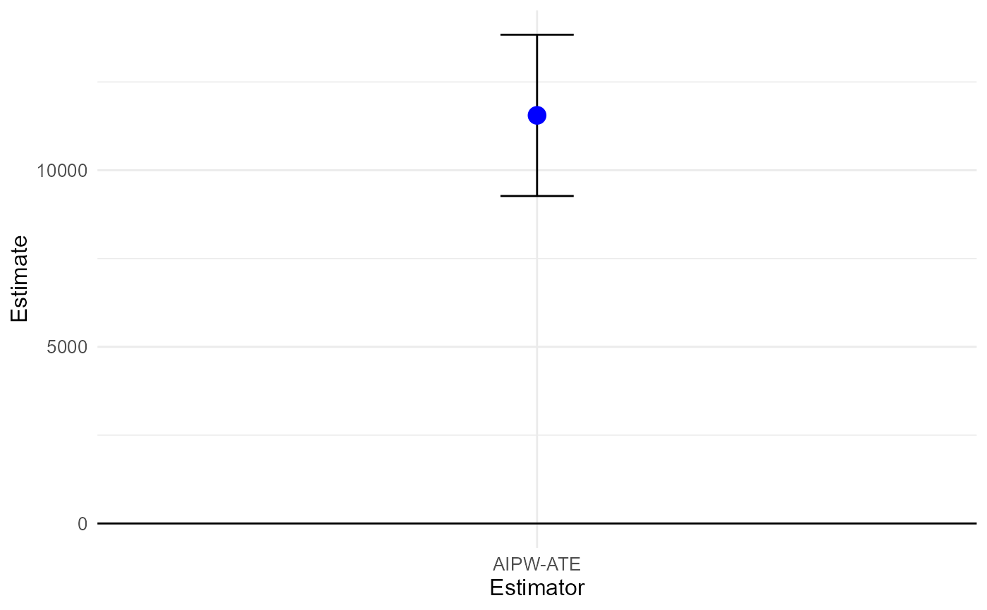

Now, we use the get_outcome_weights() method to extract the outcome weights as described in the paper.

omega_aipw = get_outcome_weights(aipw)

IPW weights

The dml_with_smoother objects also store the required components to calculate the canonical IPW weights.

D.hat = aipw$NuPa.hat$predictions$D.hat
omega_ipw = matrix(D / D.hat - (1-D) / (1-D.hat),1) / N

RA weights

The dml_with_smoother objects also store the required components to get the RA weights that are rarely used but easy to obtain.

omega_ra =  matrix(1, 1, N) %*% (aipw$NuPa.hat$smoothers$S.d1[1,,] - aipw$NuPa.hat$smoothers$S.d0[1,,]) / N

Check covariate balancing

We use the infrastructure of the cobalt package to plot Standardized Mean Differences. To do so, we need to flip the sign of the untreated outcome weights to make them compatible with the cobalt framework. This is achieved by multiplying the outcome weights by 2 \times D-1.

threshold = 0.1

love.plot(
    D ~ X,
    weights = list(
      "AIPW (Double ML)" = as.numeric(omega_aipw$omega * (2*D-1)),
      "IPW (Single ML)" = as.numeric(omega_ipw * (2*D-1)),
      "RA (Single ML)" = as.numeric(omega_ra * (2*D-1))
    ),
    thresholds = c(m = threshold),
    var.order = "unadjusted",
    binary = "std",
    abs = TRUE,
    line = TRUE,
    colors = viridis(4)
  )

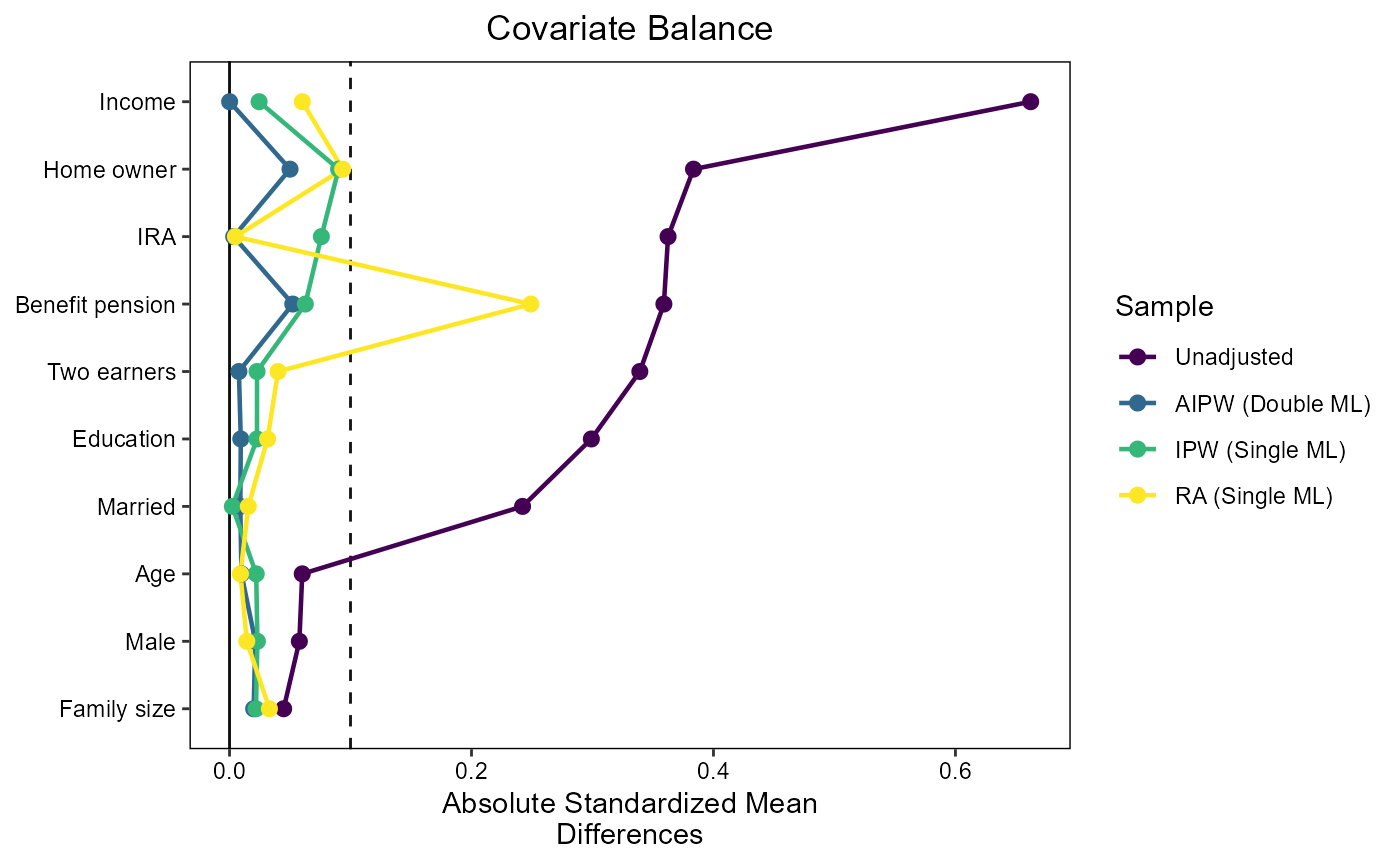
The covariate balancing of AIPW is at least as good as the balancing of IPW and RA, and in some cases substantially better. In particular, the failure of RA to balance “Benefit pension” is striking.

Conclusion

This should only serve as a small appetizer to engage with the OutcomeWeights package. If you run this on other data, please feel free to share your results via any channel. In particular, if you find qualitatively different behavior. Also please share any issues on GitHub.

Michael C. Knaus