Application 401(k) - average effects • OutcomeWeights

This notebook runs the application described in Section 5.1 of Knaus (2024). The first part replicates the results presented in the paper, the second part provides supplementary information

1. Replication of paper results

Getting started

First, load packages and set the seed:

if (!require("OutcomeWeights")) install.packages("OutcomeWeights", dependencies = TRUE); library(OutcomeWeights)
if (!require("hdm")) install.packages("hdm", dependencies = TRUE); library(hdm)
if (!require("grf")) install.packages("grf", dependencies = TRUE); library(grf)
if (!require("cobalt")) install.packages("cobalt", dependencies = TRUE); library(cobalt)
if (!require("tidyverse")) install.packages("tidyverse", dependencies = TRUE); library(tidyverse)
if (!require("viridis")) install.packages("viridis", dependencies = TRUE); library(viridis)
if (!require("gridExtra")) install.packages("gridExtra", dependencies = TRUE); library(gridExtra)

set.seed(1234)

Next, load the data. Here we use the 401(k) data of the hdm package. However, you can adapt the following code chunk to load any suitable data of your choice. Just make sure to call the treatment D, covariates X, and instrument Z. The rest of the notebook should run without further modifications.

data(pension) # Find variable description if you type ?pension in console

# Treatment
D = pension$p401
# Instrument
Z = pension$e401
# Outcome
Y = pension$net_tfa
# Controls
X = model.matrix(~ 0 + age + db + educ + fsize + hown + inc + male + marr + pira + twoearn, data = pension)
var_nm = c("Age","Benefit pension","Education","Family size","Home owner","Income","Male","Married","IRA","Two earners")
colnames(X) = var_nm

Run Double ML

In the following we run double ML with default honest random forest (tuning only increases running time without changing the insights in this application). As standard implementations do currently not allow to extract the outcome smoother matrices, the OutcomeWeights package comes with a tailored internal implementation called dml_with_smoother(), which is used in the following.

2-folds

First, we run all estimators with 2-fold cross-fitting:

# 2 folds
dml_2f = dml_with_smoother(Y,D,X,Z,
                           n_cf_folds = 2)
results_dml_2f = summary(dml_2f)

##           Estimate      SE      t         p    
## PLR        13876.4  1541.5 9.0019 < 2.2e-16 ***
## PLR-IV     12927.8  1909.3 6.7710 1.352e-11 ***
## AIPW-ATE   11681.1  1188.8 9.8258 < 2.2e-16 ***
## Wald-AIPW  11360.9  1652.3 6.8757 6.539e-12 ***
## ---
## Signif. codes:  0 '***' 0.001 '**' 0.01 '*' 0.05 '.' 0.1 ' ' 1

plot(dml_2f)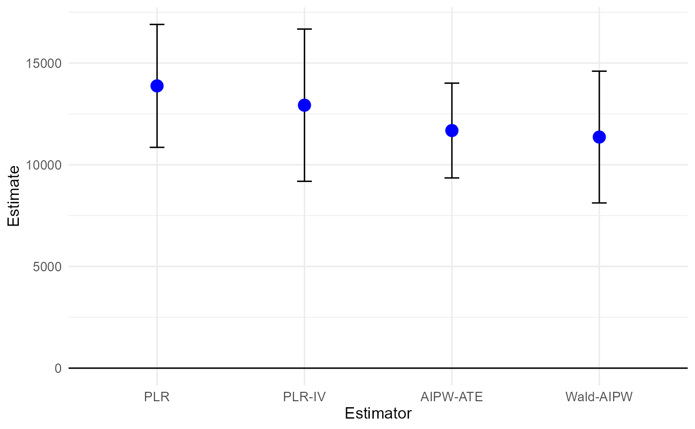

Now, we use the get_outcome_weights() method to extract the outcome weights as described in the paper. To illustrate that the algebraic results provided in the paper are indeed numerical equivalences and no approximations, we check whether the weights multiplied by the outcome vector reproduces the conventionally generated point estimates.

omega_dml_2f = get_outcome_weights(dml_2f)
cat("ω'Y replicates point etimates?", 
    all.equal(as.numeric(omega_dml_2f$omega %*% Y),
      as.numeric(results_dml_2f[,1])
    ))

## ω'Y replicates point etimates? TRUE

5-fold

Run double ML also with 5-fold cross-fitting:

# 5 folds
dml_5f = dml_with_smoother(Y,D,X,Z,
                           n_cf_folds = 5)
results_dml_5f = summary(dml_5f)

##           Estimate      SE      t         p    
## PLR        13915.5  1517.0 9.1728 < 2.2e-16 ***
## PLR-IV     13150.3  1898.5 6.9266 4.579e-12 ***
## AIPW-ATE   11530.5  1153.4 9.9972 < 2.2e-16 ***
## Wald-AIPW  11386.1  1634.5 6.9659 3.470e-12 ***
## ---
## Signif. codes:  0 '***' 0.001 '**' 0.01 '*' 0.05 '.' 0.1 ' ' 1

plot(dml_5f)

extract the weights and confirm numerical equivalence:

omega_dml_5f = get_outcome_weights(dml_5f)
cat("ω'Y replicates point etimates?", 
    all.equal(as.numeric(omega_dml_5f$omega %*% Y),
      as.numeric(results_dml_5f[,1])
    ))

## ω'Y replicates point etimates? TRUE

Check covariate balancing

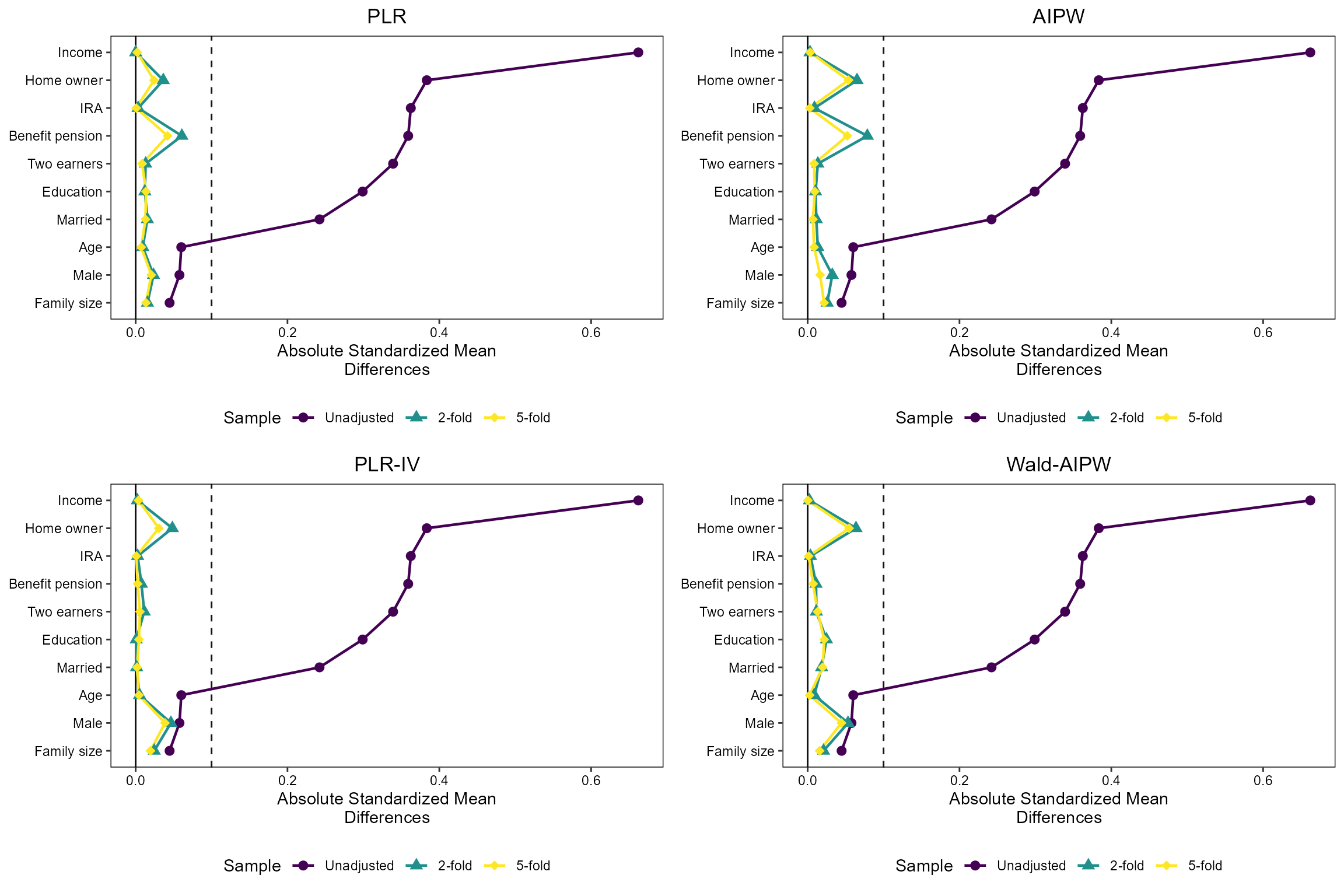
We use the infrastructure of the cobalt package to plot Standardized Mean Differences where we need to flip the sign of the untreated outcome weights to make them compatible with the package framework. This is achieved by multiplying the outcome weights by 2 \times D-1:

threshold = 0.1

create_love_plot = function(title, index) {
  love.plot(
    D ~ X,
    weights = list(
      "2-fold" = omega_dml_2f$omega[index, ] * (2*D-1),
      "5-fold" = omega_dml_5f$omega[index, ] * (2*D-1)
    ),
    position = "bottom",
    title = title,
    thresholds = c(m = threshold),
    var.order = "unadjusted",
    binary = "std",
    abs = TRUE,
    line = TRUE,
    colors = viridis(3), # color-blind-friendly
    shapes = c("circle", "triangle", "diamond")
  )
}

# Now you can call this function for each plot:
love_plot_plr = create_love_plot("PLR", 1)
love_plot_plriv = create_love_plot("PLR-IV", 2)
love_plot_aipw = create_love_plot("AIPW", 3)
love_plot_waipw = create_love_plot("Wald-AIPW", 4)
love_plot_plr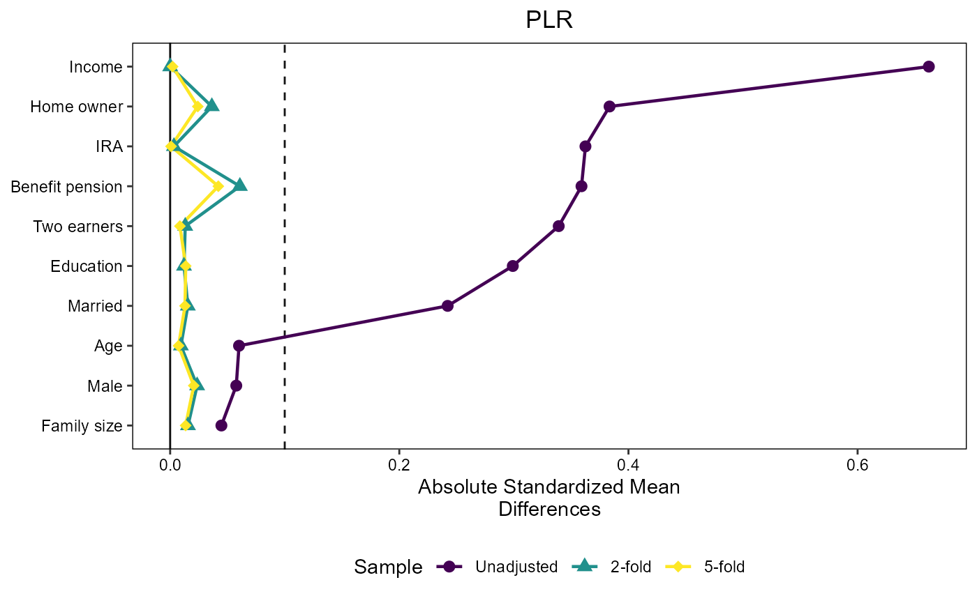

love_plot_plriv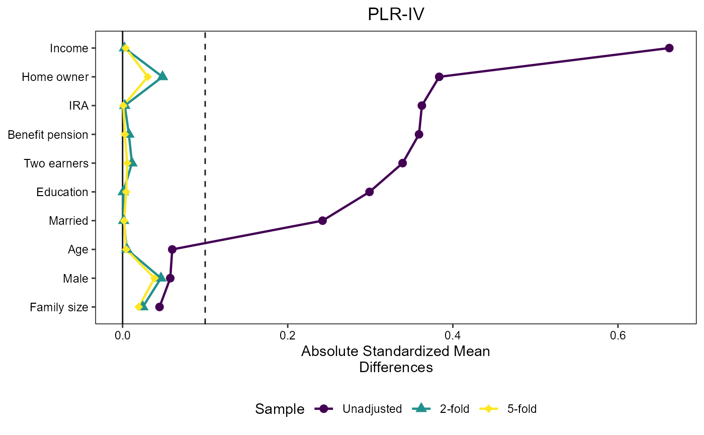

love_plot_aipw

love_plot_waipw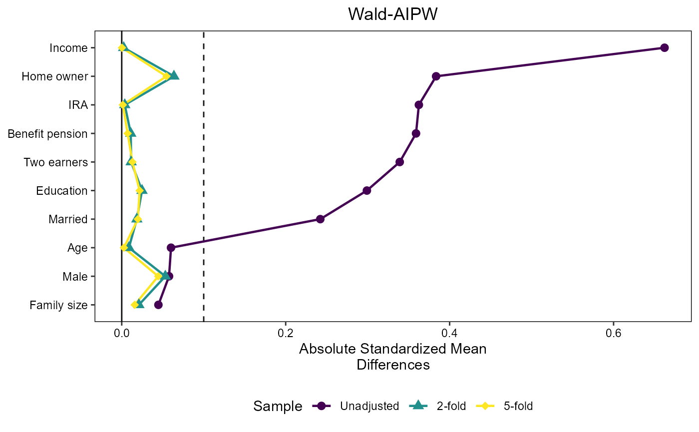

Create the combined plot that ends up in the paper as Figure 2:

figure2 = grid.arrange(
  love_plot_plr, love_plot_aipw,
  love_plot_plriv,love_plot_waipw,
  nrow = 2
)

Application 401(k) - average effects