Application 401(k) - heterogeneous effects

Michael C. Knaus

11/24

This notebook runs the application described in Section 5.2 of Knaus (2024). The first part replicates the results presented in the paper, the second part provides supplementary information

1. Replication of paper results

Getting started

First, load packages and set the seed:

if (!require("OutcomeWeights")) install.packages("OutcomeWeights", dependencies = TRUE); library(OutcomeWeights)
if (!require("hdm")) install.packages("hdm", dependencies = TRUE); library(hdm)
if (!require("grf")) install.packages("grf", dependencies = TRUE); library(grf)
if (!require("tidyverse")) install.packages("tidyverse", dependencies = TRUE); library(tidyverse)
if (!require("viridis")) install.packages("viridis", dependencies = TRUE); library(viridis)
if (!require("reshape2")) install.packages("reshape2", dependencies = TRUE); library(reshape2)
if (!require("ggridges")) install.packages("ggridges", dependencies = TRUE); library(ggridges)

set.seed(1234)

Next, load the data. Here we use the 401(k) data of the hdm package. However, you can adapt the following code chunk to load any suitable data of your choice. Just make sure to call the treatment D, covariates X, and instrument Z. The rest of the notebook should run without further modifications.

data(pension) # Find variable description if you type ?pension in console

# Treatment
D = pension$p401
# Instrument
Z = pension$e401
# Outcome
Y = pension$net_tfa
# Controls
X = model.matrix(~ 0 + age + db + educ + fsize + hown + inc + male + marr + pira + twoearn, data = pension)
var_nm = c("Age","Benefit pension","Education","Family size","Home owner","Income","Male","Married","IRA","Two earners")
colnames(X) = var_nm

Get outcome model and smoother matrix

The grf package does not save the nuisance parameter models. Thus, we could not retrieve the required smoother matrices after running causal_forest and instrumental_forest below. Therefore, we estimate the outcome nuisance model externally to pass the nuisance parameters later to the functions. As described in Section 5.2 of the paper, we run a default and a tuned version:

### Externally calculate outcome nuisance
rf_Y.hat_default = regression_forest(X,Y)
rf_Y.hat_tuned = regression_forest(X,Y,tune.parameters = "all")
Y.hat_default = predict(rf_Y.hat_default)$predictions
Y.hat_tuned = predict(rf_Y.hat_tuned)$predictions

Then, we extract the smoother matrix using get_forest_weights():

# And get smoother matrices
S_default = get_forest_weights(rf_Y.hat_default)
S_tuned = get_forest_weights(rf_Y.hat_tuned)

For illustration, check that random forest is an affine smoother by summing all smoother vectors and checking whether they sum to one:

cat("RF affine smoother?", 
    all.equal(rowSums(as.matrix(S_default)),
      rep(1,length(Y))
    ))

## RF affine smoother? TRUE

Causal forest

Run causal forest with the externally estimated outcome nuisance:

# Run CF with the pre-specified outcome nuisance 
cf_default = causal_forest(X,Y,D,Y.hat=Y.hat_default)
cf_tuned = causal_forest(X,Y,D,Y.hat=Y.hat_tuned,tune.parameters = "all")

Get the out-of-bag CATEs:

cates_default = predict(cf_default)$predictions
cates_tuned = predict(cf_tuned)$predictions

Use the new get_outcome_weights() method, which requires to pass the externally estimated outcome smoother matrix:

omega_cf_default = get_outcome_weights(cf_default, S = S_default)
omega_cf_tuned = get_outcome_weights(cf_tuned, S = S_tuned)

Observe that the outcome weights recover the grf package output:

cat("ω'Y replicates CATE point estimates (default)?", 
    all.equal(as.numeric(omega_cf_default$omega %*% Y),
      as.numeric(cates_default)
    ))

## ω'Y replicates CATE point estimates (default)? TRUE

cat("\nω'Y replicates CATE point estimates (tuned)?", 
    all.equal(as.numeric(omega_cf_tuned$omega %*% Y),
      as.numeric(cates_tuned)
    ))

## 
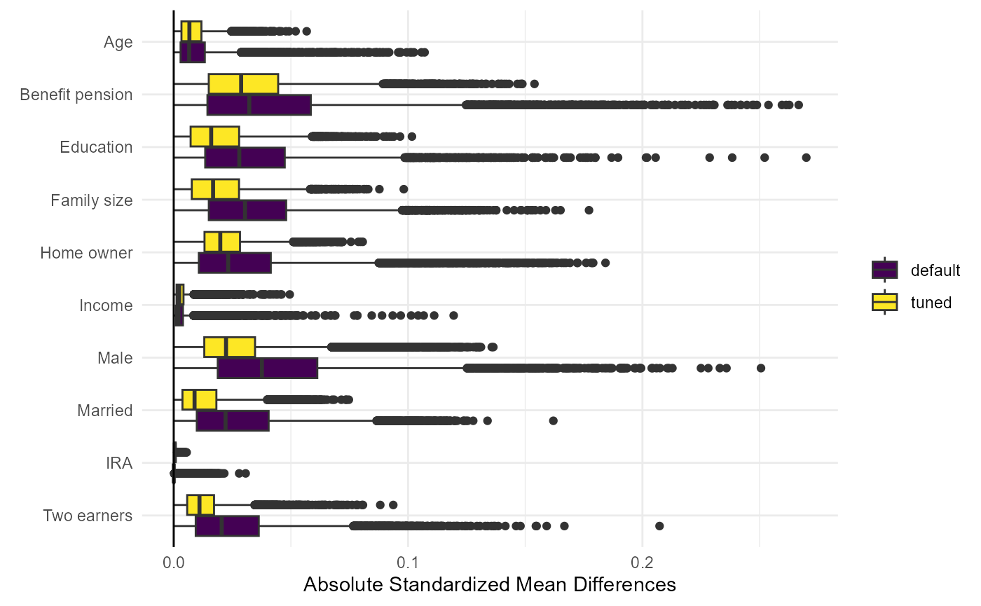
## ω'Y replicates CATE point estimates (tuned)? TRUE

Now calculate the absolute standardized mean differences and plot them for each CATE and variables (Figure 3 in paper):

cb_cate_default = standardized_mean_differences(X,D,omega_cf_default$omega,X)
cb_cate_tuned = standardized_mean_differences(X,D,omega_cf_tuned$omega,X)

smd_default = t(abs(cb_cate_default[,3,]))
smd_tuned = t(abs(cb_cate_tuned[,3,]))

# Melt the smd_default matrix to long format
df_default_long = melt(smd_default)
df_default_long$Group = "smd_default"  # Add a group identifier

# Melt the smd_tuned matrix to long format
df_tuned_long = melt(smd_tuned)
df_tuned_long$Group = "smd_tuned"  # Add a group identifier

# Combine the two data frames
df_long = rbind(df_default_long, df_tuned_long)

# Rename the columns for clarity
colnames(df_long) = c("Row", "Variable", "Value", "Group")

# Create the ggplot
figure3 = ggplot(df_long, aes(x = factor(Variable, levels = rev(unique(Variable))), y = Value, fill = Group)) +
  geom_boxplot(position = position_dodge(width = 0.8)) +
  labs(x = element_blank(), y = "Absolute Standardized Mean Differences") +
  scale_fill_manual(values = viridis(2),
                    name = element_blank(),
                    labels = c("default", "tuned")) +
  theme_minimal() +
  geom_hline(yintercept = 0, linetype = "solid", color = "black") + 
  coord_flip()
figure3